I discovered recently the Conway-s Game of Life, a celullar automaton created by matemathician John Horton Conway during 1970 to recreate natural celullar behaviours. You can found full information about it here.
Basically consist on a grid with a series of rules, you give an initial input and following the specific rules the initial grid evolve over time. The rules are this:
- Any live cell with fewer than two live neighbours dies, as if caused by under-population.
- Any live cell with two or three live neighbours lives on to the next generation.
- Any live cell with more than three live neighbours dies, as if by overcrowding.
- Any dead cell with exactly three live neighbours becomes a live cell, as if by reproduction.
This is very easy to reproduce in TP and you can have your own Game of life inside TP if you follow this little tutorial, its a cool example to learn “initiators” and “Psearch” nodes. Once you are done try to create the “Gosper Glider gun”, or oscillators, is just fun! just add an initial input and pass hours infront of the computer looking the evolution!
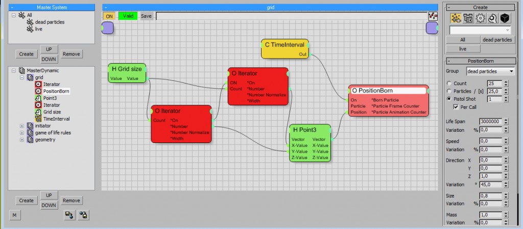
We start creating a grid of particles, we use for that “Iterator” operator. An iterator is really a cool node. Instead of output a single value, its outputing as many “integer” values as you specify on the “count” input. So If you insert in count “5″ Iterator will output from “number” the values: “0″, “1″,”2″,”3″ and “4″.If we plug this on a “Point3″ node ”x value ” and we plug this vector to the “position born” Instead of having one single position we have “5″ diferent positions where the node will emit particles. Using the “Iterator” we don-t need to create multiple position born operators. We want a single particle to every input received, so we will use “pistol Shot” to “1″ and check “Per Call”. Checking Per call Position born creates as many particles as inputs receive, If Position born receive “5″ diferent positions values (as we use Iterator) will create 5 particles, one on every input.
Using “Per Call” also means that on every frame “position born” will be active, creating on every frame new particles over the same position, we only want to create particles on the first frame, so we add a “TimeInterval” condition with “0,0″ conected to “on” so Position born will only be active the first frame.
With a single “Iterator” we create a line of particles, If we want a grid its easy, we need to create values from every single value from the first iterator. To do this we need to connect a second Iterator in “serie” with the first Iterator. Expose the “on” on the second Iterator and connect to the “On” from the first one as you see on the image. If we have “5″ number on the first Iterator and “5″ number on second Iterator, the total number of values generated is 5×5=25 values, we can connect as many Iterators as we want in serie, but be carefull since the number of values generated is exponential!
With the grid size value we can control how big we want our grid or “universe”.
We only have two groups of particles, dead particles and live particles.
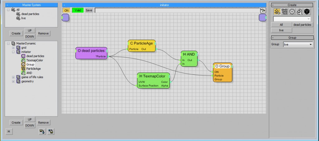
Right now we have a grid with dead particles, but we need to add an initial state, this is some live particles on the beginning from where all the system will evolve. We will send some of the dead particles to “live” particles group only on the first frame. Here I use a texmapcolor node, you can add any fractal map on it and play with the settings. On the video I create a Gosper Glider gun, and others initators states, to do that is not possible with this metode, I create instead objects where I want my particles be “live” and with a “distance” condition node I send dead particles to live. You have a lot of alternative to set up the initial state, also is possible to use a white and black map you paint by hand, or a “Pselection”.
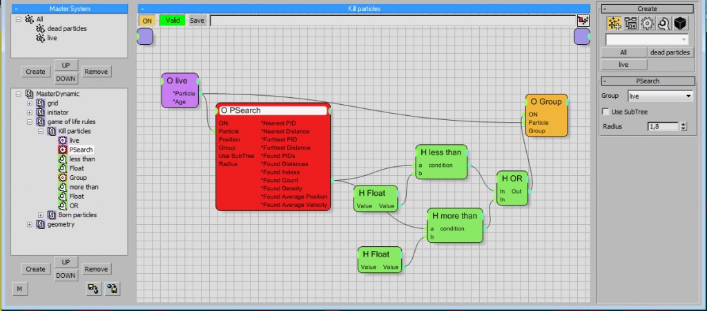
So we have to start creating the “brain” of our sistem, we have to introduce the “4″ rules created by Conway. They all refer on how many particles a single particle has around him. To Know that we use “Psearch” operator, It give a lot of information about particles near a position or another particle. For this example we will use it to know how many “Live” particles are near another “live” particle.
Create a “Psearch” Operator, and check what type of group you want to be looking at, in this case “live” group. For the radius this is important since it says how far “Psearch” will be looking around. We create the particles using an Initiator node that outputs integer values one by one, and we plug this directly to the position, so the distance between particles right now is “1″ unit. We want to be looking around the 8 particles every single particle has (left, right, top, bottom, and four corners in diagonal) The distance to a particle on the diagonal is sqrt (2)=1,41 So any number bigger than that will work, BUT! never bigger than “2″ since Psearch will start looking on particles that are not close to our particle.
Right now we can acces to the information of how many “live” particles are touching every single “live” particle. We can set now rules “1″ and “3″, sending to dead particles all particles with fewer than 2 live particles around or more than three live neighbours particles.
We will use an “expression” node for this, the expression is if(a<b,1,0) for the “less than” and if(a>b,1,0) for the “more than”. ”a” value is always the “Found count” and “b” value is “2″ on “less than” condition and “3″ on “more than” condition. You can import this expressions already done on “blackboxes”-»”conditions”. Is possible to create all of this with a single condition without using “or” node with an expression like: if(a<2,1(if(a>3,1,0)) but if you are not used to expressions the metode explained before works exactly as the simplified one and I think its easier to understand.
With all this done we only have to send our “live” particles to the group “dead” particles only when the expression is true. We have done the first and the third rule, the second rule is also done since If we don-t do anything any live cell (or particle) will be live on the next iteration.
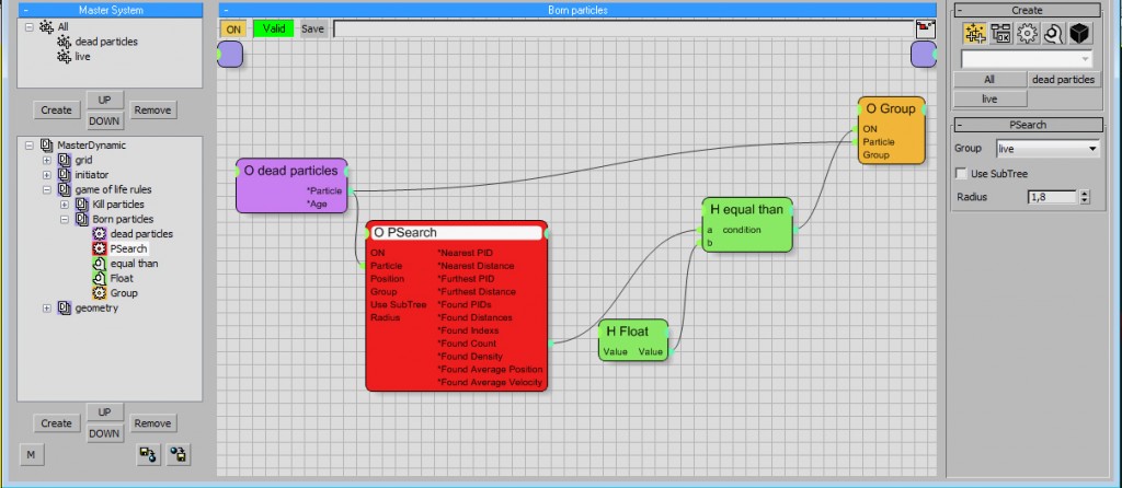
Once we did the first three rules the fourth one is similar. We have to look how many “live” particles are around a “dead” particle, and send this “dead” particle to “live” if the number is equal to “3″. The exrpression in this case is: if(a=b,1,0) with b=”3″.
Our Game of Life is complete! If you use two diferent colors for “live” and “dead” particles you will see that is working as expected. If you want you can add some geometry with diferent scales for “live” and for “dead” or what you want.
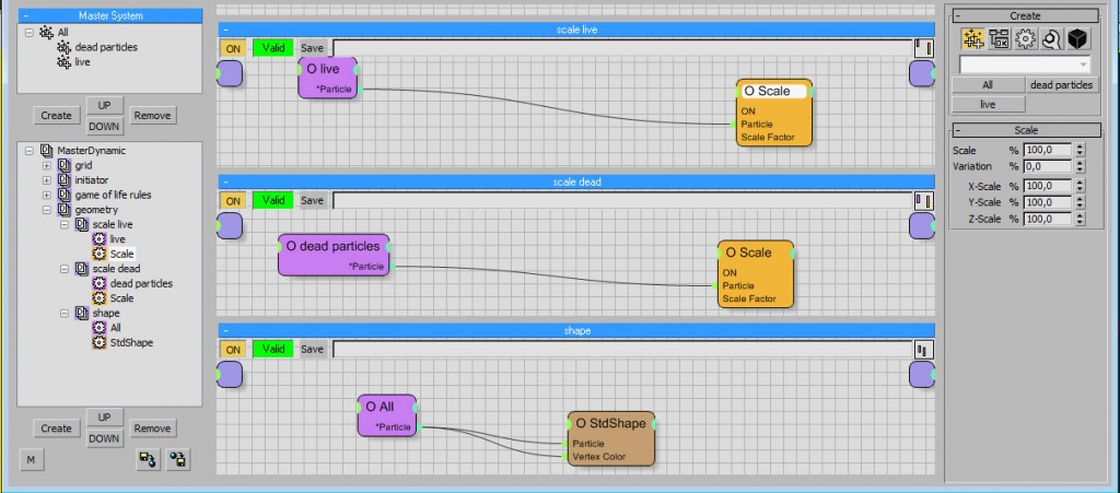
In this simple scenary, I create a cube geometry for all particles (I miss to create a condition node to only create geometry on the first frame), and a scale for “live” particles to 100% and “dead” particles to “0%”, but from here you can do what you want since the “brain” is the most important. Modify the initial distribution of life particles, create animations for your cells, create them on a 3d spaces, modify the basic Conway-s rules,… possibilities are endless!